how to make software engineering estimations
When you design a system, someone eventually asks how much storage the feature costs per year, how many requests per second the service absorbs at peak, and whether the working set fits in memory. You rarely have a benchmark or a production trace to answer with, and you still need a number before the meeting ends. The back-of-the-envelope calculation is how you produce one.
Jeff Dean, who popularized the technique at Google, describes it as a mix of thought experiments and a handful of memorized performance numbers, used to get a feel for which design meets your requirements. The output is never exact. It is an order of magnitude, and an order of magnitude is enough to kill a bad design before anyone writes code.
This article covers the three numbers every estimation rests on: the power of two for data volume, latency numbers for what the hardware costs you, and availability numbers for what an uptime promise really means. Each one comes with a worked example, and the last section puts all three together on the wallet system of a PayPal-like payment company.
the power of two
Data volume estimation starts with the units, because a mistake there is a mistake by a factor of 1,000. A byte is a sequence of 8 bits, and an ASCII character uses one byte, so a 140 character tweet stored in ASCII costs 140 bytes. Every larger unit sits one power of two away from the previous one.
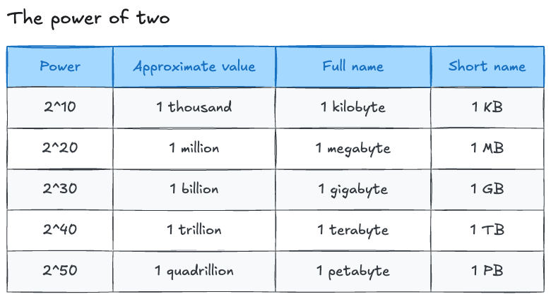
The table is the whole trick. You never multiply by 1,000 in your head, you multiply by 2^10 and read the next row.
The method has four steps.
- You estimate the size of one item, such as a message, an image, a database record, or a session.
- You estimate how many of those items the system creates or processes in a day.
- You multiply the two.
- You convert the result to KB, MB, GB, TB, or PB.
A photo sharing app makes this concrete. Assume 10 million users, one photo uploaded per user per day, and an average photo size of 2 MB:
- Photos per day = 10,000,000
- Storage per day = 10,000,000 × 2 MB = 20,000,000 MB = 20 TB
- Storage over 3 years = 20 TB × 365 × 3 ≈ 22 PB
The number itself matters less than the decision it forces. At 22 PB, no single database holds the data, so the photos go to object storage behind a CDN and the database only keeps the metadata. You reached that conclusion in four lines of arithmetic.
from daily volume to QPS
Storage answers how much you keep, and QPS, queries per second, answers how hard the system works. You get the average QPS by dividing the daily volume by 86,400, the number of seconds in a day. Traffic is never flat, so the peak QPS is commonly estimated at twice the average, and you size the servers for the peak.
The same photo app gives 10,000,000 / 86,400 ≈ 116 QPS on average, and roughly 232 QPS at peak. A few stateless application servers behind a load balancer handle that, so the interesting problem in this design is the storage, not the traffic.
latency numbers
Latency numbers tell you what an operation costs before you write a line of code. Jeff Dean published a list of the ones worth memorizing, and the relative ordering matters far more than the exact values, which keep improving with hardware.
| Operation | Latency |
|---|---|
| L1 cache reference | 0.5 ns |
| Branch mispredict | 5 ns |
| L2 cache reference | 7 ns |
| Mutex lock and unlock | 100 ns |
| Main memory reference | 100 ns |
| Compress 1 KB with a fast algorithm | 10 µs |
| Send 2 KB over a 1 Gbps network | 20 µs |
| Read 1 MB sequentially from memory | 250 µs |
| Round trip inside the same datacenter | 500 µs |
| Disk seek | 10 ms |
| Read 1 MB sequentially from the network | 10 ms |
| Read 1 MB sequentially from disk | 30 ms |
| Round trip from California to the Netherlands | 150 ms |
Four conclusions come out of that table, and they drive most architecture decisions you make.
- Memory is fast and disk is slow. Reading 1 MB from disk costs about 120 times more than reading it from memory, which is the entire argument for a cache.
- Compression is cheap and the network is expensive. Compressing 1 KB costs 10 µs, and sending it costs an order of magnitude more, so you compress data before it goes over the wire.
- A disk seek costs 10 ms, so sequential access beats random access by a wide margin, and the data layout on disk is worth designing.
- A cross-continent round trip costs 150 ms, more than a human notices. Cross-region calls belong on a background path, not in the request path.
availability numbers
High availability is the ability of a system to stay operational over a period of time, and it is measured as the percentage of that period during which the service responds. A service at 100% has zero downtime, and real services land between 99% and 99.999%. When a provider commits to a number in a contract, the contract is called a service level agreement, or SLA, and it also defines the credit the customer receives when the provider misses the target.
Each extra nine divides the downtime budget by ten.
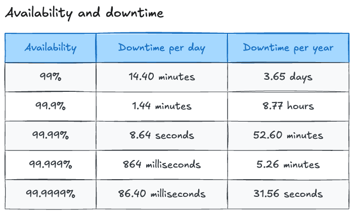
The table is worth reading twice, because the intuition here is usually wrong. Availability of 99.9% sounds close to perfect, and it still allows 8.77 hours of downtime per year, a full working day of outage. Removing most of those hours means moving to 99.99%, which buys you redundancy across availability zones, automated failover, and an on-call rotation that answers at 3 a.m. Every nine you promise has a price, so the target belongs to the business, not to the architecture diagram.
putting the three together
The wallet system of a PayPal-like company exercises all three numbers at once. A wallet holds a balance, a transaction moves money between two wallets, and the ledger records every movement forever. The estimation starts with assumptions, and writing them down explicitly is part of the technique, because a reviewer who disagrees with your conclusion usually disagrees with an assumption.
- The company has 400 million wallets.
- One user in ten transacts on a given day, which gives 40 million active wallets per day.
- Each active user makes 2 transactions per day on average.
- Each user checks a balance or a history 10 times for every payment they send.
- Regulation forces the company to keep the ledger for 7 years.
The traffic comes first, and payments have an asymmetry worth catching early:
- Transactions per day = 40,000,000 × 2 = 80,000,000
- Average write QPS = 80,000,000 / 86,400 ≈ 1,000
- Peak write QPS ≈ 2 × 1,000 = 2,000
- Average read QPS ≈ 10 × 1,000 = 10,000
Black Friday and payday cycles push a payment system well past a factor of two, so a retail peak of 10,000 writes per second is a fair planning number rather than 2,000. The reads dominate anyway, which already tells you the read path deserves its own caching layer.
The storage follows from the size of one ledger entry. A double-entry ledger writes a debit and a credit per transaction, and one row carries two wallet identifiers, an amount, a currency, a status, timestamps, and an idempotency key. Rounding to 500 bytes per row with its indexes:
- Rows per day = 80,000,000 × 2 = 160,000,000
- Ledger per day = 160,000,000 × 500 bytes = 80 GB
- Ledger over 7 years = 80 GB × 365 × 7 ≈ 200 TB
The hot balances are a separate calculation, and the power of two answers it in one line. A balance record of 100 bytes for 40 million daily active wallets costs 40,000,000 × 100 bytes = 4 GB, which fits in memory on a single cache node. The latency table explains why that matters: a balance read from memory costs 250 µs per MB against 30 ms from disk, so the balance check that runs 10,000 times per second belongs in a cache and never touches the ledger.
The latency budget closes the argument. A payment API that answers in 300 ms has room for a datacenter round trip at 500 µs and a durable disk commit at a few milliseconds, and it has no room for a cross-region round trip at 150 ms, which alone eats half the budget. The write path therefore stays inside one region and the replicas in other regions receive the data asynchronously.
Availability sets the last constraint, and here the money makes the case. At 80 million transactions per day, one hour of downtime drops roughly 3.3 million transactions, so a 99.9% target with its 8.77 hours of annual downtime is indefensible for a payment company. The target is 99.99% or better, which is why the design carries automated failover and a multi-zone deployment.
None of these numbers is large by internet standards. A ledger of 200 TB fits in a sharded relational cluster, and 10,000 writes per second at peak is unremarkable. The estimation did not tell you the system is hard, it told you where the difficulty actually sits: durability, correctness, and uptime, not raw scale.
rules of thumb
A few habits make these estimations fast and defensible.
- You round aggressively, because the goal is an order of magnitude. A day has 86,400 seconds, and rounding it to 100,000 costs you 15% of accuracy and saves you a minute of mental arithmetic.
- You write the assumptions above the calculation, so a reviewer can challenge the input instead of the output.
- You label every unit, since the difference between a bit and a byte is a factor of 8, and the difference between GB and TB is a factor of 1,000.
- You state the decision the number leads to. An estimate that changes nothing was a waste of time.